Main | Mathematical Methods | CRAVA User Guide |  Download

---

Inversion | Background model | Wavelet | Prior Correlations | Optimal Well Locations | Facies Probabilities | Rock Physics

---

To calculate facies probabilities from inverted elastic parameters we must first establish a link between the elastic parameters from inversion and facies. There are several ways to do this, and we have listed the four most realistic in the table below.

Different methods for establishing a relation between elastic parameters and facies.

Approach	Frequency Control	Inversion Correlation	Alignment	Predictions
Rock physics	No	No	Yes	Optimistic
Low-pass filtered elastic well logs	Yes	No	Yes	Optimistic
Inversion	Yes	Yes	No	Pessimistic
Parameter filtered elastic well logs	Yes	Yes	Yes	Realistic

 

Figure 1: Acoustic impedance residuals calculated from blocked raw logs plotted against corresponding Vp/Vs residuals (left), the same plot, but with logs high-cut frequency filtered to 40Hz (middle), and the same logs but filtered using frequency and correlation information from inversion (right).

 

First, we may establish the link using a rock physics models. This way we avoid any alignment problems, but we get no frequency control and get to use no correlation information from the inversion. A prediction obtained this way tends to be too optimistic, but if there are no well logs available, this is our only option.

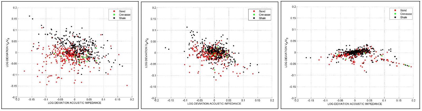
Second, we may filter the elastic well logs using a low-pass filter, and use these filtered logs and facies logs to make a density estimation of $p\left({\mathbf{\mu }}_{m|d_{obs}}\right|f)$, where f is the facies. This gives us frequency control and proper alignment, but again there are no correlation information from the inversion included, and the predictions become to optimistic. The frequency filtering of well logs is illustrated in Figure 1.

Third, we may set up the probability density for an elastic responds given the facies directly from the inverted elastic parameters. This way we get both frequency control and correlation information included, but we get no alignment information, and the predictions become to pessimistic. Finally, we may establish the density using elastic parameters from well logs, but filter these using frequency and correlation information obtained from the inversion. Since we only use well logs to establish the density estimates, we get no  alignment problems, and in total, this gives us realistic facies predictions. How the inversion-based filtering differs from the pure frequencybased filtering mentioned above is illustrated in Figure 1.

The link between facies and elastic parameters that we eventually are interested in is p(f_i|µ_m|d,i), where f_i is the facies at location i and µ_m|d,i is the inversion result at the same location. To establish this link, we must first establish a link between the well logsmand the expectation given the seismic data µ_m|d(obs).

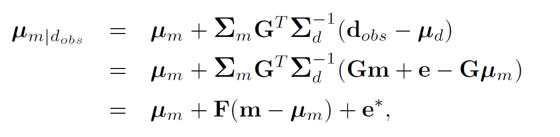
where

 

Figure 2. To the left, the posterior sand probability calculated without undefined facies. In the middle, the sand probability when undefined facies is introduced. To the right, the posterior probability for undefined facies.

 

The operator F is used to filter the well logs and obtain an estimate of the expected inversion values m*. For each facies, we then do a density estimation of p(µ_m|d(obs) | f) for each possible facies value f using m and facies logs. The density estimation is done using a kernel smoothing approach, and by using the distribution of e* as our kernel, we get an unbiased estimate of this distribution. Finally, we find the facies probability:

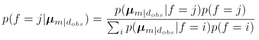
where p(f = i) is the prior probability of facies i. This probability is then computed for each facies and each cell in the grid, with µ_m|d(obs) given by the inversion results. Far away from wells, the estimates will not be reliable, and we introduce an undefined facies to show such areas. Denoting the likelihood of this undefined facies p(u), the facies probabilities are now calculated as

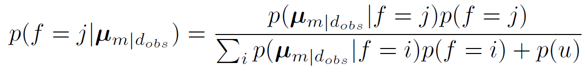
where p(u) is uniform over the area, and low compared to the likelihood for facies when we are close to data.

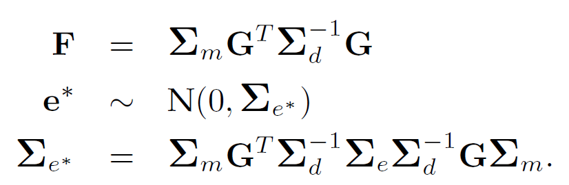
In Figure 2 the effect of the undefined facies in a reservoir consisting of sand and shale is illustrated. The three figures show cross plots of well observations of $\rho$ against Vp combined with a probability map shown as a Colo coded map.

In the left figure, we show the probability of sand before the undefined facies has been introduced. Note how combinations of $\rho$ and Vp which are far away from any well observations, as for instance (Vp, $\rho$) = (2000m/s, 2.25g/cm3), may still lead to a facies prediction of sand equal to one. This is not realistic.

In the middle figure, the undefined facies has been introduced, and whenever we get far away from combinations of $\rho$ and Vp for which we have no well observations, the probability for sand now decreases to zero. This does not mean that there is no chance of finding sand at the current spot, only that we have no data support to tell us what facies we might find. Similarly, the probability of finding shale will also be zero.

In the right figure, we show the probability of the undefined facies. This is zero around well observations, and gradually increases to one as the distance to observations increase. The probability of shale may be extracted from these figures since p(sand) + p(shale) + p(undefined) = 1.

 

Facies probabilities in Crava

How facies probabilities are calculated depends on the input to CRAVA. If facies probabilities from rock physics is requested, CRAVA will make synthetic wells from the rock physics models. If rock physics is not used and there are real  wells supplied in the input, CRAVA will make use of these. In both cases, the wells are filtered and used to make a smooth probability distribution from the histogram of observed values.

Trends

With rock physics, it is also possible to have zero, one or two trends. Trend minimum and maximum values are specified by the user. If the maximum trend value is equal to the minimum value, this is interpreted as having no trend. Each trend axis is divided in 20 bins. Since the grids in general are very large, it is advantageous to keep the number of dimensions low. When there are either one or two trend dimensions, CRAVA will automatically reduce the three elastic  dimensions to the two components that are best resolved by seismic. By minimizing the expression

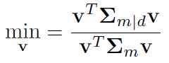
once, the best resolved feature is found. The second best feature is found by minimizing the same expression but with the additional constraint of being uncorrelated to the first component. This amounts to choosing the eigenvectors of ${\mathbf{\Sigma }}_m^{-1}{\mathbf{\Sigma }}_{m|d}$ sorted in increasing order of the corresponding eigenvalues. However, the use of trends will increase the number of numerical grids in use in CRAVA:

1. With real wells and no rock physics: the wells are filtered and a 3D grid (where the threedimensions represent the three elastic parameters) is filled with the observed values.
2. If facies probabilites from rock physics is requested:

• With no trend, a 3D grid is filled with values from the synthetic wells.
• With one trend, the three elastic dimensions are reduced to two dimensions and 20 (the number of bins in the trend dimension) 2D grids (actually 3D grids where only two dimensions are in use) are filled.
• With two trends, the three elastic dimensions are reduced to two dimensions and 202 = 4000 (the number of bins in the trend dimension) 2D grids (actually 3D grids where only two dimensions are in use) are filled.

Sythetic wells

When rock physics is used, 10 synthetic wells, each of minimum length 100 bins, is simulated per combination of trend parameters. If no trends are used, 10 such wells are simulated. The synthetic wells are made as follows:

1. If the length of the well is less than 100 bins, draw one of the relevant facies from a uniform distribution (no correlation with the facies above).
2. Draw a facies length from a geometric distribution with expectation 10 ms.
3. Generate a well sample of this length by calling the functionality described in section 2.8 and add this piece to the well.

Well filtering and smoothing

The final probability distribution is smoothed with the seismic uncertainty. This uncertainty is calculated using the prior and posterior spatial covariance for the elastic parameters in the well. For both real and synthetic wells, the distribution of the error in the inversion is calculated as

Each well is filtered independently. The bins in the probability grids (one per facies) are then filled with the values from the wells and a Gaussian distribution with covariance in the elastic dimensions from the well filter is created. The facies  probability grids are then convoluted with the Gaussian distribution by FFT. This gives $\widehat{p}\left({\widehat{\mathbf{m}}}_i\right|f_i,\mathbf{z}).$

Calculating facies probabilities

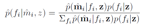
The final lithology prediction is computed as

The uncertainty-level is part of the input to CRAVA and specifies the likelihood for undefined lithologies. This value is scaled according to the size of the grid, but will result in a high probability for undefined facies if the relevant point is not close to one of the modes in the distribution.