- Inversion
- Inversion
Main | Mathematical Methods | CRAVA User Guide | Download
Inversion | Background model | Wavelet | Prior Correlations | Optimal Well Locations | Facies Probabilities| Rock Physics
The CRAVA program uses the Bayesian linearised AVO inversion method of Buland et al. (2003) to take the uncertainty in seismic amplitude data into account. Since we only use amplitude data, we will from here on use the term seismic data for these. The seismic data are described using multi-normal distributions, and modelled as the seismic response of the earth model plus an error term. The earth model and error term are modelled as multi-normal distributions in which spatial coupling is imposed by correlation functions. Using a Bayesian setting, prior models for the earth and error terms are set up based on prior knowledge obtained from well logs, and the process of seismic inversion is reduced to that of finding a posterior distribution for the earth given the seismic data. The linearised relationship between the model parameters and the AVO data, makes it possible to obtain the posterior distribution analytically.
The posterior distribution for earth model parameters Vp (pressure-wave velocity), Vs (shearwave velocity), and (density), gives a laterally consistent seismic inversion. The lateral correlation can follow the stratigraphy of the inversion interval by following the top and/or base of the inversion volume, but can also be specified independently using a correlation surface. As a consequence of the spatial coupling, the solution in each location depends on the solutions in all other locations. From the posterior distribution the best estimate of the model parameters and a corresponding uncertainty can be extracted. Moreover, since the distribution is Gaussian, kriging can be used to match the well data, and the posterior covariance can be computed. This spreads full frequency information in an area around the wells. Full frequency realizations can be generated by sampling from the posterior distribution. A set of such realizations represents the uncertainty of the inversion.
AVO
Amplitude versus offset (AVO) inversion can be used to extract information about the elastic subsurface parameters from the angle dependency in the reflectivity, see e.g., Buland et al. (1996); Hampson and Russell (1990); Lörtzer and Berkhout (1993); Pan et al. (1994). In practice, and especially for 3-D surveys, linearised AVO inversion is attractive since it can be performed with use of moderate computer resources. Prior to a linearised AVO inversion, the seismic data must be processed to remove nonlinear relations between the model parameters and the seismic response. Important steps in the processing are the removal of the move-out, multiples, and the effects of geometrical spreading and absorption. The seismic data should be pre-stack migrated, such that dip related effects are removed. After pre-stack migration, it is reasonable to assume that each single bin-gather can be regarded as the response of a local 1-D earth model. The benefits of pre-stack migration before AVO analysis are discussed in Brown (1992); Buland and Landrø (2001); Mosher et al. (1996). It is further assumed that wave mode conversions, interbed multiples and anisotropy effects can be neglected after processing. Ideally, the pre-stack gathers are also transformed from offsets to reflection angles. Offset gathers are often close to angle gathers, so we can use these, but if the inversion area is thick, this will give more noise in the CRAVA model.
Seismic Model
The seismic response of an isotropic, elastic medium is completely described by the three material parameters
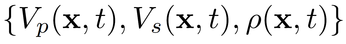
where the vector x gives the lateral position (x,y), and t is the vertical seismic travel time.
The weak contrast approximation by Aki and Richards (1980), relates the seismic reflection coefficients to the elastic medium, and is a linearization of the Zoeppritz equations. A continuous version of this approximation is given by Stolt and Weglein (1985):
Equation 1: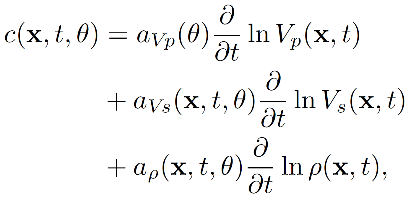
where theta is the PP reflection angle, and
Equation 2: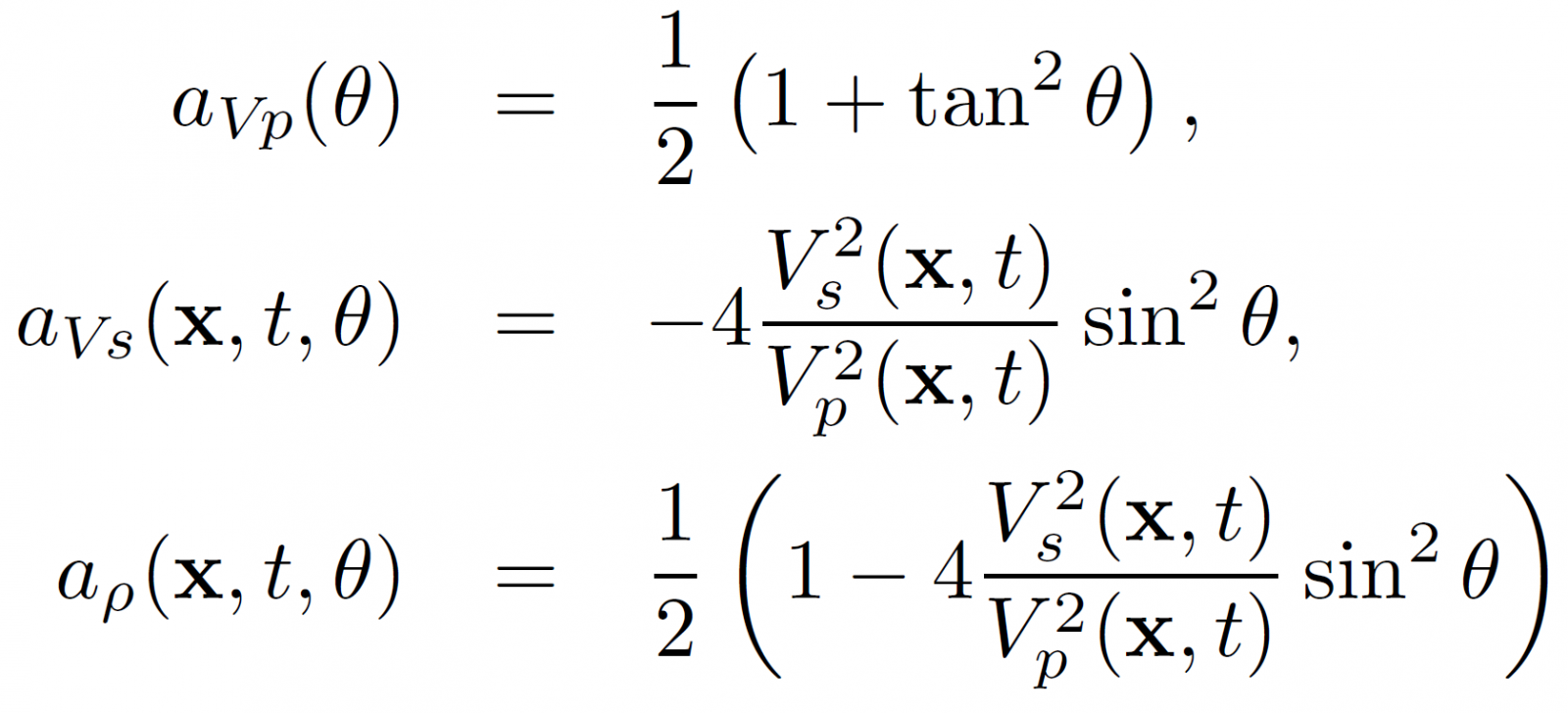
for PP reflections, and
Equation 3: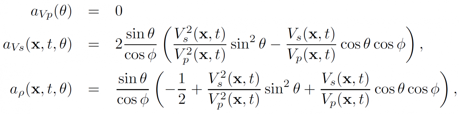
for PS reflections. Here, is the PS reflection angle, given by .
These equations are linearised by replacing the ratio Vs(x, t)/Vp(x, t) with a constant value Vp/Vs when computing the coefficients.
The seismic data are represented by the convolutional model
Equation 4: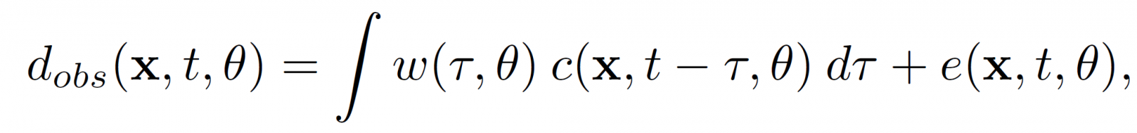
where w is the wavelet, and e is an angle and location dependent error term. The integral is the synthetic seismic. The wavelet can be angle dependent, and can vary laterally according to scale and shift maps. The wavelet is assumed to be stationary within a limited target window.
The signal-to-noise ratio is defined as the ratio of the energy of the data to the energy of the noise as given in Equation 4 above, that is,
Equation 5: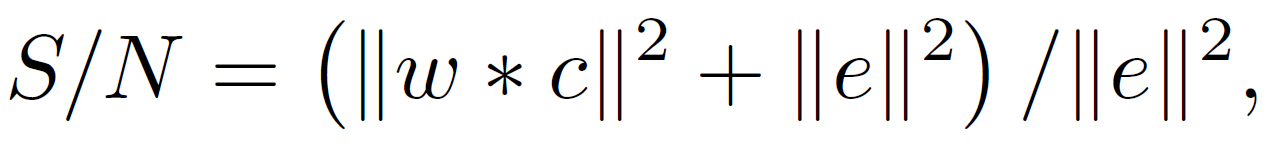
where the operator * denotes the convolution. Since the error is independent of the synthetic seismic, the energy form the synthetic seismic and the noise can simply be added. Note that there also exists another definition of the S/N ratio where the noise energy is not included in the enumerator.
Statistical model
The elastic parameters Vp(x, t), Vs(x, t), and are assumed to be log-normal random fields. This means that the distribution
Equation 6:is multi-normal or multi-Gaussian, that is,
Equation 7:where µm(x,t) gives the expectation of m(x,t) and where gives covariance structure.
We assume that the covariance function is stationary and homogeneous (i.e., translationally invariant), and can be factorised as
Equation 8: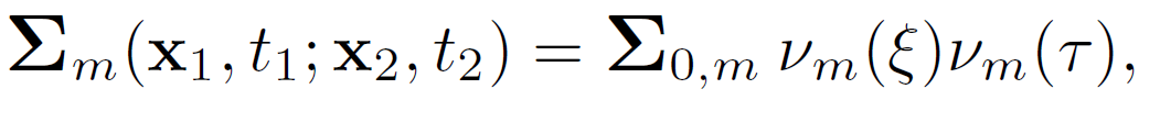
where and are correlation functions depending on the lateral and temporal distances and , respectively, and is a matrix of the variances and covariances of ln(Vp), ln(Vs) and ln(). Any covariance structure giving a positive definite may be used.
If we let m and dobs be discrete representations of m(x, t) and in a time interval, Equation 4 may be written in matrix notation as
Equation 9: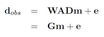
where W is the matrix representation of the wavelets, A is a matrix encompassing discrete representations of the coefficients aVp, aVs, and arho, D is a differential matrix and G = WAD. The error matrix e is a time discretization of the error vector
Equation 10: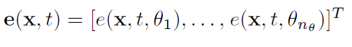
and is assumed to be zero-mean coloured Gaussian noise, that is,
Equation 11:The covariance of the error vector is
Equation 12:where is an covariance matrix containing the noise variances for the different reflection angles on the diagonal, and the covariances between the angles off the diagonal. Furthermore, and are lateral and temporal correlation functions.
Since the relationship between the reflection coefficients and the elastic parameters given in Equation 1 is linear, and the elastic parameters are assumed Gaussian distributed, the reflection coefficients become Gaussian. Moreover, since the convolution is a linear operation and we have assumed a Gaussian error model, the seismic data given in Equation 4 are also Gaussian distributed.
For the time-discretized seismic data dobs, this gives us the multi-normal distribution
Equation 13: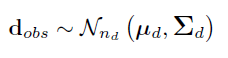
where
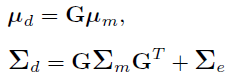
where all vectors and matrices are time-discretized.
This means that the simultaneous distribution for m and dobs is Gaussian, and that the distribution for m given dobs can be obtained analytically using standard theory for Gaussian distributions:
Equation 14: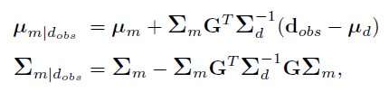
where µd is the expected observation, that is, the seismic response of µm, and is the covariance matrix between logarithmic parameters and observations. See Buland and Omre (2003) for a detailed description on how to compute these.
The computations given in equations above involves the inverse of
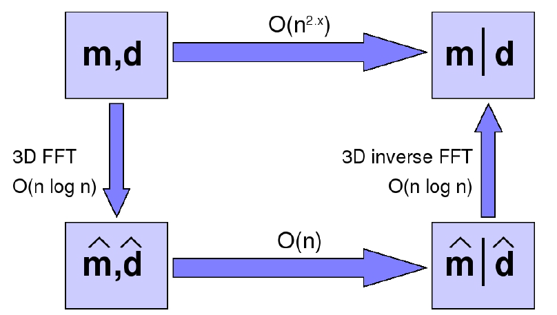
This seems to require that d is stationary, which would imply that the wavelet must be the same everywhere. However, we can divide out the wavelet from Equation 9 to obtain
Equation 15: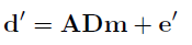
where d' is the data divided by the wavelet, and e' is the error divided by the wavelet. The details of how we do this division is given in Section 2.6.1 in the manual. Note that we now assume that the noise after division, e' is stationary. Since we assume that a seismic response only depends on the reflections in that trace, this division can be done trace by trace. This assumption relies on a rather smooth seismic response, so the lateral variations in the wavelet should be smooth. We have chosen to restrict the local wavelet changes to only allow local temporal shift and amplitude scaling. We can also work around the stationary noise assumption, and allow e' to vary laterally. This is done by utilising the nature of a Bayesian solution, which always is a tradeoff between the prior and the posterior with noise free data. By finding the posterior for a minimal noise, we can then interpolate between this solution and the prior to find an appropriate solution for the local noise level. When doing this, we ignore the lateral correlation, so we require constant noise level in each trace, since the conditional correlations inside a trace are much stronger than between traces.
Buland, A. and Omre, H. (2003). Bayesian linearized AVO inversion. Geophysics, 68:185–198.
Buland, A., Landrø, M., Andersen, M., and Dahl, T. (1996). AVO inversion of troll field data. Geophysics, 61:1589–1602.
Hampson, D. and Russell, B. (1990). AVO inversion: Theory and practice. pages 1456–1458.
Lörtzer, G. J. M. and Berkhout, A. J. (1993). Linearized AVO inversion of multicomponent seismic data. In Castagna, J. and Backus, M., editors, Offset-Dependent Reflectivity – Theory and practice of AVO analysis, pages 317–332. Soc. Expl. Geophys.
Pan, G. S., Young, C. Y., and Castagna, J. P. (1994). An integrated target-oriented prestack elastic waveform inversion: Sensitivity, calibration, and application. Geophysics, 59:1392–1404.
Brown, R. L. (1992). Estimation of AVO in the prescence of noise using prestack migration. pages 855–888.
Buland, A. and Landrø, M. (2001). The impact of common offset migration on porosity estimation by AVO inversion. Geophysics, 66:755–762.
Mosher, C. C., Keho, T. H., Weglein, A. B., and Foster, D. J. (1996). The impact of migration on AVO. Geophysics, 61:1603–1615.
Aki, K. and Richards, P. G. (1980). Quantitative Seismology: Theory and Methods. W. H. Freeman and Co.
Stolt, R. H. andWeglein, A. B. (1985). Migration and inversion of seismic data. Geophysics, 50:2458–2472.
Christakos, G. (1992). Random field models in earth sciences. Academic Press Inc., San Diego.
 Hvordan komme til NR
 Del på sosiale media
 Personvernerklæring