- Background Model

Main | Mathematical Methods | CRAVA User Guide | Download

The expectation µ_m is usually referred to as the background model. As the seismic data do not contain information about low frequencies, a background model is built to set the appropriate levels for the elastic parameters in the inversion volume. To identify this level, we can plot the frequency content of the seismic traces in the available wells, and identify lowest frequency for which seismic data contains enough energy to carry information.

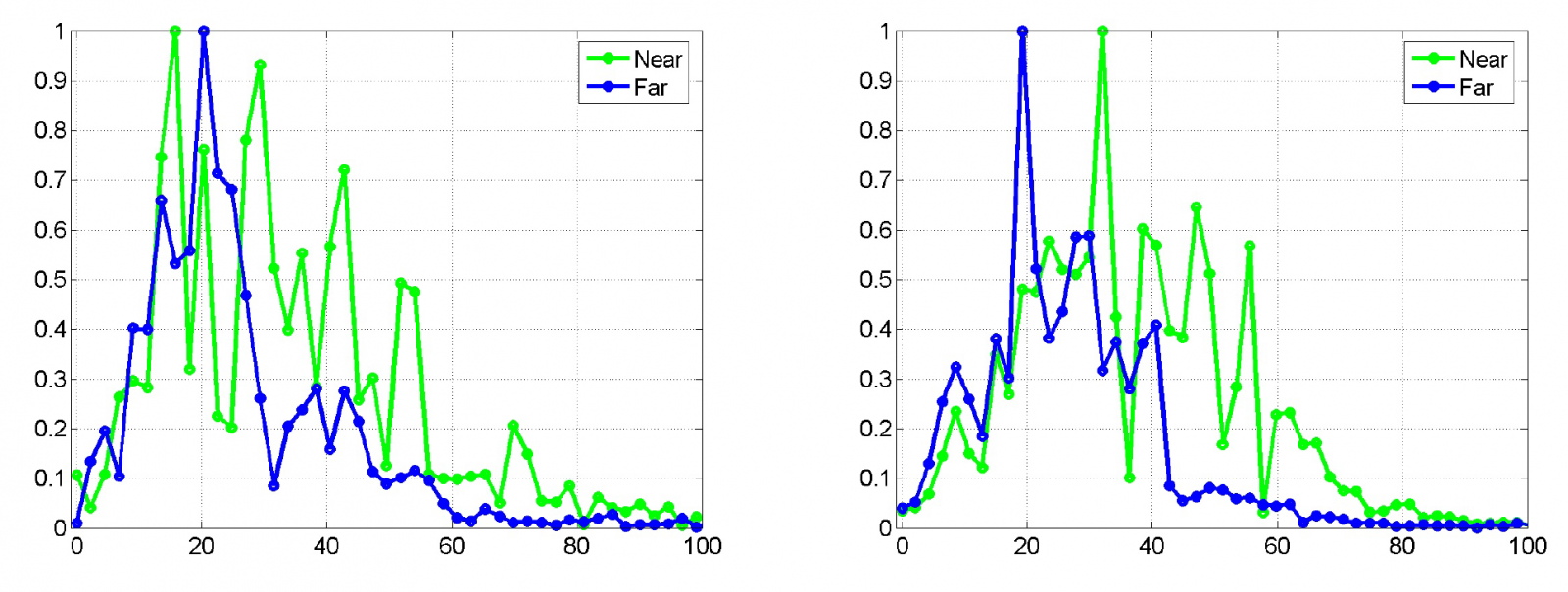
In Figure 1, we have plotted the frequency content in the seismic data in two different wells. The green curve gives the frequency content in the near stack and the blue curve gives the frequency content in the far stack. These plots show that the seismic data contain little energy below 5–6Hz, and the purpose of the background model is to fill this void.

Figure 1: The frequency content of the seismic traces in two different wells. The frequency content of the near and far stacks are shown as green and blue curves respectively.

The estimation of the background model is made in two steps. First, we estimate a depth trend for the entire volume, and then we interpolate well logs into this volume using kriging. The estimation will by default contain information up to 6Hz, but this high-cut limit can be adjusted using by user as input to crava with a high-cut-background-modelling keyword.

When identifying the depth trend, it is important that the wells are appropriately aligned. The alignment is defined by the time interval surfaces specified as input, or alternatively, the correlation direction surface. It is important that the alignment reflects the correlation structure (deposition/compaction), and if the time surfaces are either eroding or on-lapped, one should consider specifying the correlation direction separately using the <correlation-direction> keyword.

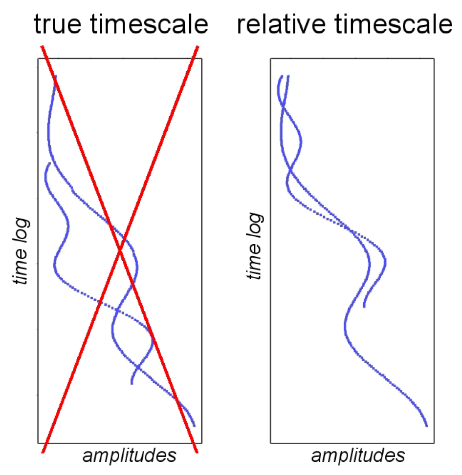
In Figure 2, we show two well logs aligned according to deposition and according to the true time scale. Evidently, an incorrect trend will be identified if the true vertical depth is used. The size of the error will depend on the stratigraphy.

Figure 2: Well logs aligned according to true time scale (left) and according to stratigraphic depth (right).

Assuming properly aligned wells, the trend extraction starts by calculating an average log value for each layer. This average is calculated for the Vp, Vs, and ρ well logs and is based on all available wells. The estimation uses a piecewise linear regression, rather than the more straightforward arithmetic mean or moving average, as these measures are sensitive to the amount of data available. The piecewise regression has the additional advantage that it can give trend estimates also outside the interval for which we have data available.

For the linear regression we require a minimum of 10 data points behind each estimate. In addition, we require that the minimum number of data points must also be at least 5*Nwells. This way we ensure that data points from different time samples are always included. Alternatively, the regression would reduce to an arithmetic mean whenever there are 10 or more wells available. If we enter a region with no data points available at all, the minimum requirements are doubled. To get the right frequency content in the depth trends, the regression values are eventually frequency filtered to 6Hz.

Figure 3: Well log values plotted against grid layer number for Vp (left) and (right). The blue circles show log values, the green curve is a piecewise linear regression of the these values, and the red curve is the regression values filtered to 6Hz.

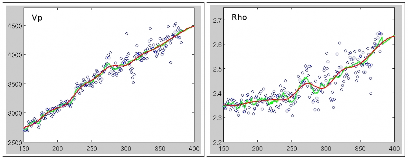
The trend extraction process is illustrated in Figure 3 for the Vp and logs of a field with six wells. Note that the plots are oriented with layers as abscissa and log values as ordinate. The blue circles represent log values from any wells, the green curve is the piecewise linear regression of these values, and the red curve is the frequency filtered log that will be used as a depth trend. Note that the green curve is slightly erratic, especially, as we enter the region (below reservoir) where there are no data points available. This shift, which is clearly observed for the density, arises as we stabilise the estimate by requiring twice as many data points behind each estimate.

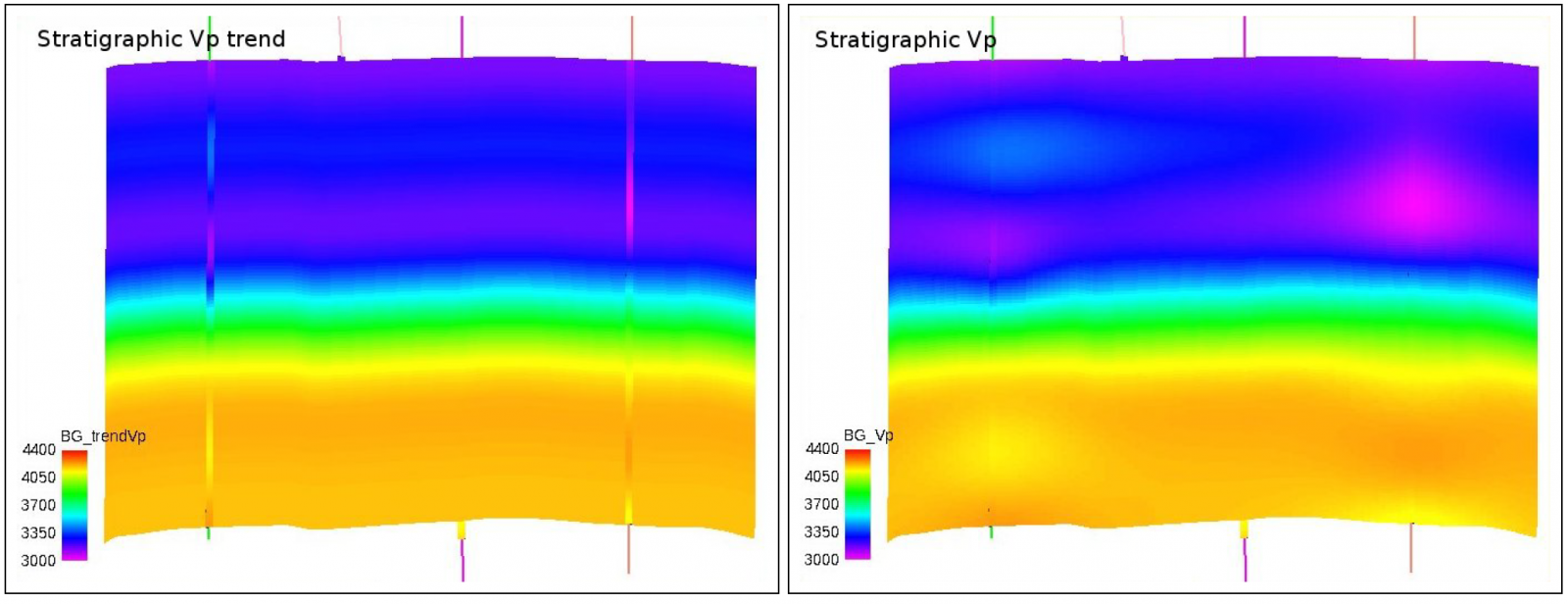
Figure 4: Vp depth trend (left) and final background model (right). Well logs of Vp, high-cut filtered to 6Hz, are shown for comparison.

When the inversion volume has been filled with the depth trend, we interpolate it with 6Hz filtered well logs, to ensure that the background model will match in wells. A cross section of the resulting background model for Vp is illustrated in the right part of Figure 4. To the left is the corresponding depth trend. For comparison the well logs of Vp has plotted in both illustrations. Note how the wells influence the volume in a region around the well. Ideally, the background model should be as smooth as possible, and a Gaussian variogram model with relatively long ranges may seem an obvious choice. This model is too smooth, however, and should be omitted as it often give parameter over- and undershooting away from wells.

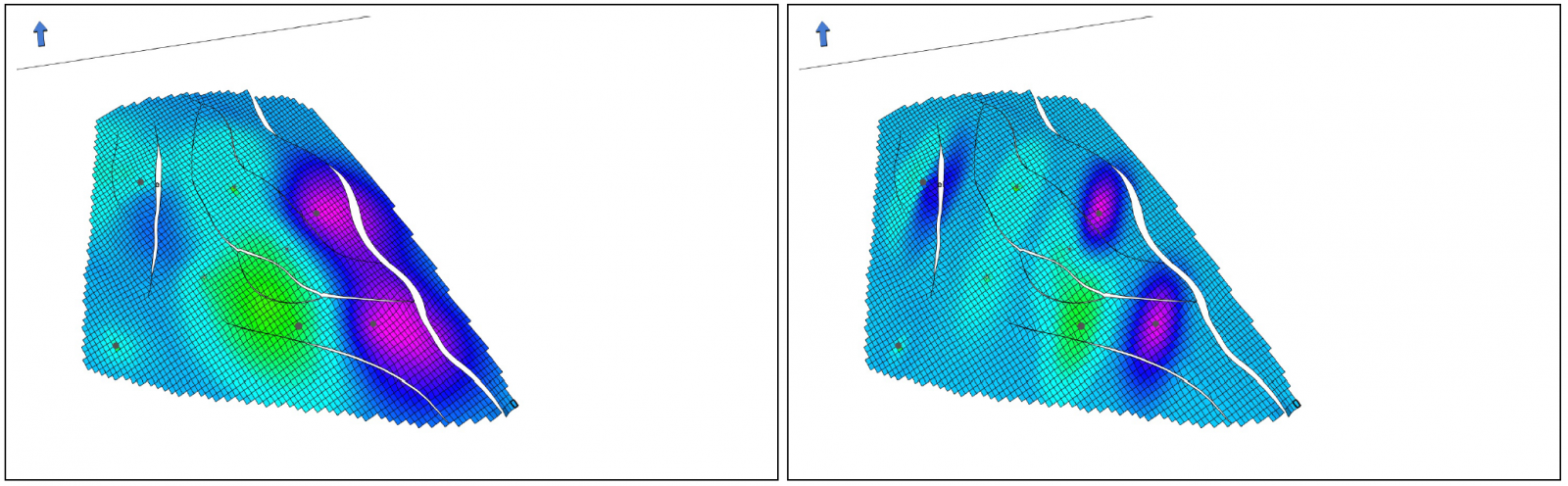
If the user wants detailed control of the variogram used in the kriging here, the command <lateral-correlation> can be used under <background> in <prior-model>. This variogram will then be used when kriging wells, and allows the user to control the well influence radius and anisotropy. If the ranges given are not equal, the well will have different influence range along and across the azimuth direction. The azimuth range is typically largest, giving a larger well influence in this direction. This can make sense in depositional environments, where the well influence in the depositional direction generally will be larger than across. The value for the range is how far away a point should be from a well before it is no longer influenced by the well. Examples of the effect of using this keyword is shown in Figure 5.

Figure 5: Lateral cross sections of two different background models, where only the <lateral-correlation> variogram has changed between them.

Multizone background model

When estimating the multizone background model the reservoir is divided into several horizontal zones defined by surfaces in the inversion volume. In each zone, a local background model is made by estimating a depth trend for the zone volume, then kriging well logs to the depth trend. The settings for interval uncertainty and erosion priority are set under <multiple-intervals>. The background model in each zone contains frequencies up to 6Hz, but the frequency content is higher in the transitions between the zones. These higher frequencies will, however, contain information about the locations of the zones; hence they contain important prior information. Higher uncertainty gives smoother background models with lower frequency.

Background from Rock Physics

When rock physics models are used, the background model is generated using these. Each facies is defined as a rock, possibly containing trends using the rock physics template. The resulting background model is generated as a weighted average of the rock models, where the weights are the corresponding facies prior-probabilities given as input.

If well logs are available, the elastic parameters in the background model, i.e. the expectations, and the corresponding precision/variance, can be modelled from data, respectively. Moreover, if there exist appropriate reference parameters, like two-way-time and/or stratigraphic depth, it is also possible to model the elastic parameters as 1- or 2-dimensional functions of the provided reference parameters. In principle, these reference parameters can be almost anything, as long as they provide some underlying structure to the problem at hand. Also, note that it is possible to combine different models, in the sense that we might model the trend as constant while the variance is a two dimensional surface that depends on a 2-dimensional reference parameter, see subsection 3.5.2.3 in the manual for more details.

The expectation is fitted using a modified version of a standard local linear regression implementation with a Gaussian kernel. In short, what distinguishes this implementation from those more commonly used, is that it will provide more stable estimates outside the main support of data. This is achieved by gradually increase the bandwidth in the kernel as the method extrapolate away from the main support of the observations. This happens, however, at just the right rate to make a smooth transition to a standard linear model in regions far away from the centre of the observations. The bandwidth aims at, in all locations, to give a ‘effective sample sizes’, i.e. the total weight of the kernel at a given point, that matches that in the main support of the data, with a bandwidth set to optimize the asymptotic properties (limiting minimize mean square error), under the assumption that the observations are uniformly distributed over the domain. The estimated variances are a weighted averages between the estimated global variance and estimates from a standard implementation of a kernel smoother with a Gaussian kernel. The weights, used in the mixture, are the effective sample sizes. The selected bandwidth is kept fixed and is the same as used to estimate the expectation inside the main support of the data. This construction removes a rather undesirable feature of the standard kernel smoother, which estimates a variance that is too low, or zero, in regions with few observations.

Search form

Search form