- Inversion
- Inversion
Main | Mathematical Methods | CRAVA User Guide | Download
XML Model | Inversion | Estimation | Forward modelling | Rock Physics | Facies Predictions
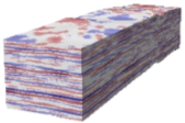
Inversion mode will invert the seismic data to elastic parameter (Vp, Vs and Density) and/or facies probabilities.
Minimum input is a seismic cube, volume and a well. All other missing data will be estimated.
There are two option, prediction and simulation of the elastic parameters.
Inversion is run by specifying inversion with the <mode> keyword under <actions>,
<actions>
<mode> inversion </mode>
</actions>
Prediction
Prediction gives "the most probable" elastic properties given the data. The prediction is unique given the seismic data and the assumptions about the wavelet and the physical models.
<actions>
<mode> inversion </mode>
<inversion-settings>
<prediction> yes </prediction>
</inversion-settings>
</actions>
Example of inversion with prediction model files can be downloaded here.
Simulation
Stochastic simulation (Monte Carlo) is an alternative to prediction. There are two main reasons for using stochastic simulation:
- The uncertainty (variability) in the inversion is considered important.
- The small scale spatial structure below seismic resolution is considered important.
This is given with <simulation> under <inversion-settings>, where <seed> and <number-of-simulations> can be specified, e.g.
<actions>
<mode> inversion </mode>
<inversion-settings>
<simulation>
<seed> 123456 </seed>
<number-of-simulations> 10 </number-of-simulations>
</simulation>
</inversion-settings>
Stochastic simulated realizations are not unique and will span all possibilities within the constraints of seismic data and the assumptions on seismic wavelet and physical models. Note that the average of a large set of simulations (>50) will be identical to the prediction.
Example of inversion with simulation model file can be downloaded here.
Singlezone inversion
Single zone inversion is specified by using the keyword <interval-two-surfaces> under <output-volume>, e.g:
<project-settings>
<output-volume>
<interval-two-surfaces>
<top-surface>
<time-file> TopSurface.storm </time-file>
</top-surface>
<base-surface>
<time-file> BaseSurface.storm </time-file>
</base-surface>
<number-of-layers> 100 </number-of-layers>
</interval-two-surfaces>
</output-volume>
</project-settings>
Multizone inversion
To perform inversion in multiple zones the <multiple-intervals> under <output-surfaces>, e.g.
<project-settings>
<output-volume>
<multiple-intervals>
<top-surface>
<time-file> TopSurface.storm </time-file>
</top-surface>
<interval>
<name> Interval1 </name>
<base-surface>
<time-value> 2000 </time-value>
<erosion-priority> 2 </erosion-priority>
</base-surface>
</interval>
<interval>
<name> Interval2 </name>
<base-surface>
<time-file> BaseSurface.storm </time-file>
<erosion-priority> 3 </erosion-priority>
</base-surface>
</interval>
</multiple-intervals>
</output-volume>
</project-settings>
Where more <interval> tags can be added to include additional zones/intervals. The inversion is done separately for each interval and finally combined to a final grid, which consist of the first top surface and the last base surface. The resolution used in the output grid is taken from the smallest resolution from all intervals.
Each interval given in <multiple-intervals> are defined by a name. This name is used as a reference when other interval based settings are set. These are <vp-vs-ratio>, <correlation-direction>, <parameter-autocovariance>, <prior-probabilities> and <volume-fractions>.
One must also set the <erosion-priority> which defines which surface to be used when two surfaces intersect. All the base surfaces need to be given a unique priority. The surface with highest priority is given erosion priority two (top surface has priority one), while the surface with lowest priority is given priority n, where n is equal to the number of surfaces.
One can also set the <uncertainty> for all base surfaces, this is used to smooth results across border when they are merged to a final grid. To represent uncertainties between intervals a beta distribution with parameters alpha and beta equal to 2 is used. The distribution is symmetric around its center, being the surface between the intervals. The limits in the Beta distribution, given by the keyword <uncertainty>, is the distance of the uncertainty in ms in each direction from the surface.
Example of multizone inversion model file can be downloaded here.


 How to get to NR
 Share on social media
 Privacy policy