- Prior Correlations
- Prior Correlations
Main | Mathematical Methods | CRAVA User Guide | Download
Inversion | Background model | Wavelet | Prior Correlations | Optimal Well Locations | Facies Probabilities| Rock Physics
Since we model the covariance structure as separable, we have collapsed the full time dependent covariances between parameters into:
-
parameter covariance matrix
 ,
, -
lateral correlation vector

-
temporal correlation vector
 .
.
We estimate the correlations by first blocking the wells into the grid, and then do standard correlation estimation using
The parameter covariance matrix is simply estimated by using the covariances at time lag 0. When rock physics models are used, the parameter covariance matrix is calculated from the expectation vector and parameter covariance matrix for each rock model weighted with the corresponding prior facies probability using standard statistical models. If trends are included in the rock physics models, the parameter covariance matrix is calculated in each reservoir position. The resulting parameter covariance matrix is then calculated as the average over these covariance matrices.
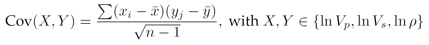
In Figure 1, we show cross plots of the parameter residuals () for a sample field. The depicted distributions look similar to bivariate normal distributions, which supports the normal distribution assumptions made for the statistical model. If there are no Vs logs available, the prior Vs variance will be set equal to twice the Vp variance, and their covariance will be set equal to zero. This is unrealistically low, but will result in a more uncertain Vp than otherwise, which we feel is correct given that we are unable to estimate its relationship with Vs and its variance in this case.
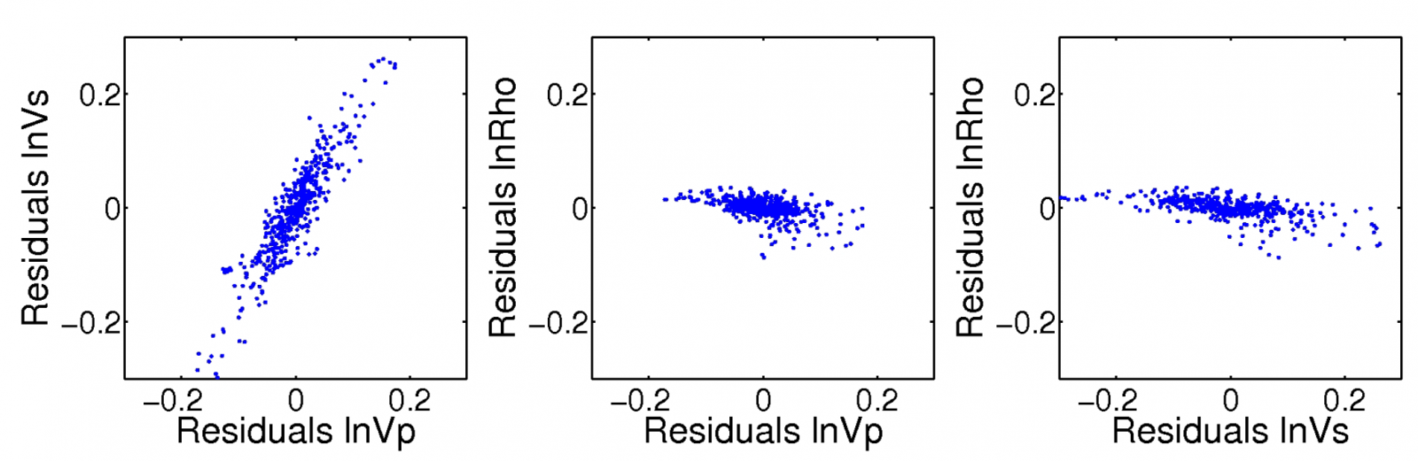
The temporal correlation is estimated from the remaining lags in the well logs as depicted in Figure 2. The temporal correlation will be a weighted average of the estimates made for all three elastic parameters.
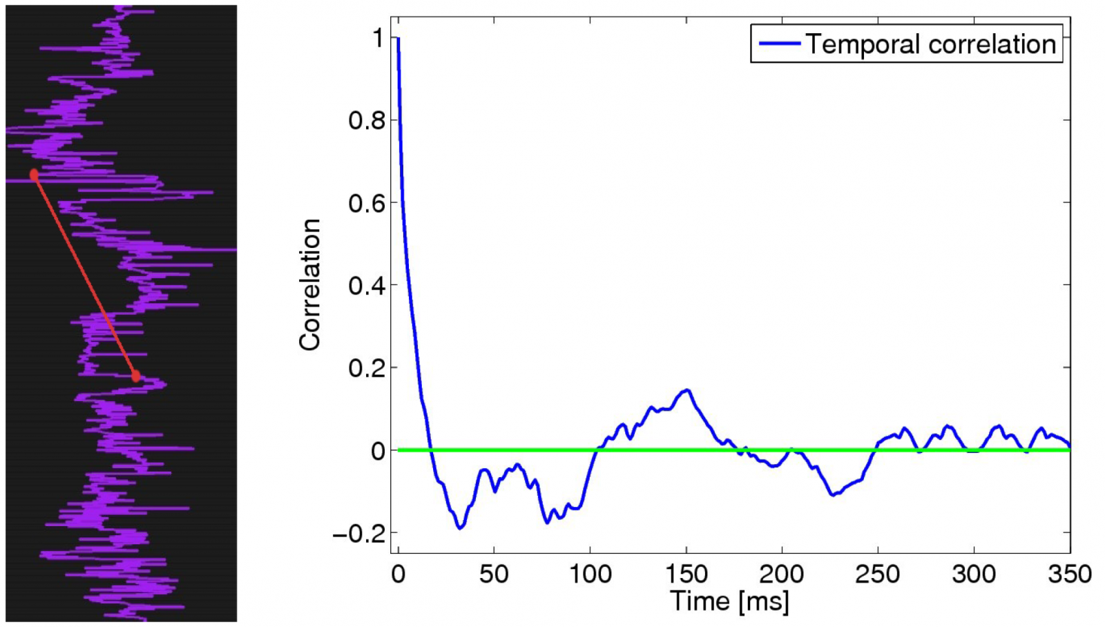
While the covariance matrix and the temporal correlation can be readily estimated from well data, this is not the case for the lateral correlation, unless there are a large number of wells available. The lateral correlation is therefore normally chosen parametric. There is an option in CRAVA to estimate the lateral correlation from seismic data, but these estimates are not made relative to stratigraphy and tend to grossly underestimate the correlation. Using a parametric correlation function is therefore encouraged. In Figure 3, we have depicted an exponential correlation function and the lateral correlation structure this kind of function gives rise to.
 Hvordan komme til NR
 Del på sosiale media
 Personvernerklæring